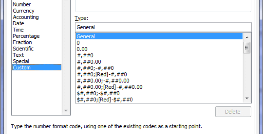
Excel and other spreadsheet programs use number formats to display the contents in cells a certain way.
This makes life easier for the user and subsequently any viewer of that spreadsheet later especially if it’s printed out.
How Excel displays numbers and text
When you start with a new spreadsheet, you learn that a spreadsheet is made up of columns that are given letters and rows that are given numbers. Where these columns and rows cross are referred to as cells and are located using the column letter and row number, so the first cell is A1.
This cell arrangement is the basis of spreadsheets from the early programs that used them. However, how the cell contents is displayed is set in the number format system in Excel and initially starts with General, so a number 1 will show as 1.
If you want to show that number as a currency, you highlight the cell with the 1 in it and click the currency button and you now have £1.00
Nice and simple, and Excel has loads of different number formats to choose from but they can be limited, so you can create your own number format.
This is different from formulas that work with the contents of different cells to give a calculated result.
Custom field types
When you create your own custom field type, Excel has a basic rule for you to follow:
There are 4 forms that the cell can contain, and are handled in different ways:
- Positive numbers (any number larger than 0)
- Negative numbers (any number less than 0)
- Zero or blank entries
- Text entries
Each type you create consists of the rules for each of these forms and is laid out as:
positive;negative;zero;text
You are also allowed up to two conditional statements, so you could have:
[Red][<10]0;[Blue][>=10]0
What this will do is when the positive number in the cell is below 10, it will be red but if the number is above or equal to 10 it will be blue. You cannot use more than 2 conditional statements in a number format however, if you need more, you do this with conditional formatting which relies on formulas within the cell themselves.
Accounting with red and black
I use the following format for my accounts, because I like to see both the cell showing whether the amount is positive in black or negative in red, but also using the format of accounting, where the £ sign is left aligned and the amount is right aligned.
_-£* #,##0.00_-;[Red]-£* #,##0.00_-;_-£* “-“??_-;_-@_-
So basically, this interprets as:
_-£* (space) tells Excel to display a space before the £ sign of the width of a minus sign, then show the £ sign and then pad it the full width of the cell (left aligned)
#,##0.00 tells Excel that we will display the number with two decimal places and any number that has less than two decimal places, add the appropriate zeros, so 10 becomes 10.00
Finally, we add another space at the end.
For negative numbers, we change the cell colour to red and apply the same rule, but we include a – symbol just before the £ sign to show the number is negative.
If the cell is empty or contains a zero, we apply the space and then use the ?? notation for Excel to display the cell in decimal alignment before displaying a text minus sign, followed by the space. The result being £ – for the cells that contain zero or are blank.
Lastly, if the cell contains text, we apply the space at the beginning, then insert the @ text placeholder and then the space after.
Red and black numbers
I also use a simpler approach with numbers:
0;[Red]-0;0;@
So we display the number if it’s positive, if it’s negative we show the number as red and with a negative sign. If it’s zero or blank, show zero and if it’s text we display the text.

